Outline

Multiway ANOVA

MANOVA

Beyond two factors

We can consider multiple factors $A$, $B$, $C$, $\dots$ with respectively $n_a$, $n_b$, $n_c$, $\dots$ levels and with $n_r$ replications for each.

The total number of treatment combinations is

Full three-way ANOVA model

Each cell of the cube is allowed to have a different mean

$$\begin{array}{c}\underset{\text{response}cell}{Y_{ijkr}{\mu }_j}=\underset{\text{cell mean}}{{\mu }_{ijk}}+\underset{\text{error}cell}{{\epsilon }_{ijkr}{\mu }_j}\end{array}$$ with ${\epsilon }_{ijkt}$ are independent error term for

• row $i$
• column $j$
• depth $k$
• replication $r$

Parametrization of a three-way ANOVA model

With the sum-to-zero parametrization with factors $A$, $B$ and $C$, write the response as

$$\begin{array}{cc}\underset{\text{theoretical average}}{E\left(Y_{ijkr}\right)}& =\underset{\text{global mean}}{\mu }\\ & +\underset{\text{main effects}}{{\alpha }_i+{\beta }_j+{\gamma }_k}\\ & +\underset{\text{two-way interactions}}{(\alpha \beta {)}_{ij}+(\alpha \gamma {)}_{ik}+(\beta \gamma {)}_{jk}}\\ & +\underset{\text{three-way interaction}}{(\alpha \beta \gamma {)}_{ijk}}\end{array}$$

Example of three-way design

Interaction plot

The microwave popcorn experiment

What is the best brand of microwave popcorn?

• Factors
• brand (two national, one local)
• power: 500W and 600W
• time: 4, 4.5 and 5 minutes
• Response: weight, volume, number, percentage of popped kernels.
• Pilot study showed average of 70% overall popped kernels (10% standard dev), timing values reasonable
• Power calculation suggested at least $r=4$ replicates, but researchers proceeded with $r=2$...

ANOVA table

data(popcorn, package = 'hecedsm')
# Fit model with three-way interaction
model <- aov(percentage ~ brand*power*time,
             data = popcorn)
# ANOVA table - 'anova' is ONLY for balanced designs
anova_table <- anova(model) 
# Quantile-quantile plot
car::qqPlot(model)Copy Code

Quantile-quantile plot

All points fall roughly on a straight line.

Code for interaction plot

popcorn |> 
   group_by(brand, time, power) |>
   summarize(meanp = mean(percentage)) |>
ggplot(mapping = aes(x = power, 
                     y = meanp, 
                     col = time, 
                     group = time)) + 
  geom_line() + 
  facet_wrap(~brand)Copy Code

Interaction plot

No evidence of three-way interaction (hard to tell with $r=2$ replications).

Variance decomposition for balanced designs

Analysis of variance table for the 3-way model

Omitting terms in a factorial design

The more levels and factors, the more parameters to estimate (and replications needed)

• Costly to get enough observations / power
• The assumption of normality becomes more critical when $r=2$!

It may be useful not to consider some interactions if they are known or (strongly) suspected not to be present

• If important interactions are omitted from the model, biased estimates/output!

Guidelines for the interpretation of effects

Start with the most complicated term (bottom up)

• If the three-way interaction $ABC$ is significative:
  • don't interpret main effects or two-way interactions!
  • comparison is done cell by cell within each level
• If the $ABC$ term isn't significative:
  • can marginalize and interpret lower order terms
  • back to a series of two-way ANOVAs

Marginalization vs main effects

Marginalization means that we reduce the dimension of the problem, e.g., we transform a three-way ANOVA into a two-way ANOVA by collapsing over a dimension.

Main effects are the effects of factors $A$, $B$, $C$ (i.e., row, column and depth effects).

What contrasts are of interest?

• Can view a three-way ANOVA as a series of one-way ANOVA or two-way ANOVA...

Depending on the goal and if the interactions are significative or not, could compare for variable $A$

• marginal contrast ${\psi }_A$ (averaging over $B$ and $C$)
• marginal conditional contrast for particular subgroup: ${\psi }_A$ within $c_1$
• contrast involving two variables: ${\psi }_{AB}$
• contrast differences between treatment at ${\psi }_A\times B$, averaging over $C$.
• etc.

See helper code and chapter 22 of Keppel & Wickens (2004) for a detailed example.

Effects and contrasts for microwave-popcorn

Following preplanned comparisons

• Which combo (brand, power, time) gives highest popping rate? (pairwise comparisons of all combos)
• Best brand overall (marginal means marginalizing over power and time, assuming no interaction)
• Effect of time and power on percentage of popped kernels
• pairwise comparison of time $\times$ power
• main effect of power
• main effect of time

Preplanned comparisons using emmeans

Let $A$=brand, $B$=power, $C$=time

Compare difference between percentage of popped kernels for 4.5 versus 5 minutes, for brands 1 and 2

$$H_0:({\mu }_{1.2}-{\mu }_{1.3})-({\mu }_{2.2}-{\mu }_{2.3})=0$$

library(emmeans)
# marginal means
emm_popcorn_AC <- emmeans(model, 
                          specs = c("brand","time"))
contrast_list <- 
  list(
    brand12with4.5vs5min = c(0, 0, 0, 1, -1, 0, -1, 1,0))
contrast(emm_popcorn_AC,  # marginal mean (no time)
         method = contrast_list) # list of contrastsCopy Code

Preplanned comparisons

Compare all three times (4, 4.5 and 5 minutes)

At level 99% with Tukey's HSD method

• Careful! Potentially misleading because there is a brand * time interaction present.

# List of variables to keep go in `specs`: keep only time
emm_popcorn_C <- emmeans(model, specs = "time")
pairs(emm_popcorn_C, 
      adjust = "tukey", 
      level = 0.99, 
      infer = TRUE)Copy Code

Motivational example

From Anandarajan et al. (2002), Canadian Accounting Perspective

This study questions whether the current or proposed Canadian standard of disclosing a going-concern contingency is viewed as equivalent to the standard adopted in the United States by financial statement users. We examined loan officers’ perceptions across three different formats

Alternative going-concern reporting formats

Bank loan officers were selected as the appropriate financial statement users for this study.

Experiment was conducted on the user’s interpretation of a going-concern contingency when it is provided in one of three disclosure formats:

1. Integrated note (Canadian standard)
2. Stand-alone note (Proposed standard)
3. Stand-alone note plus modified report with explanatory paragraph (standard adopted in US and other countries)

Multivariate response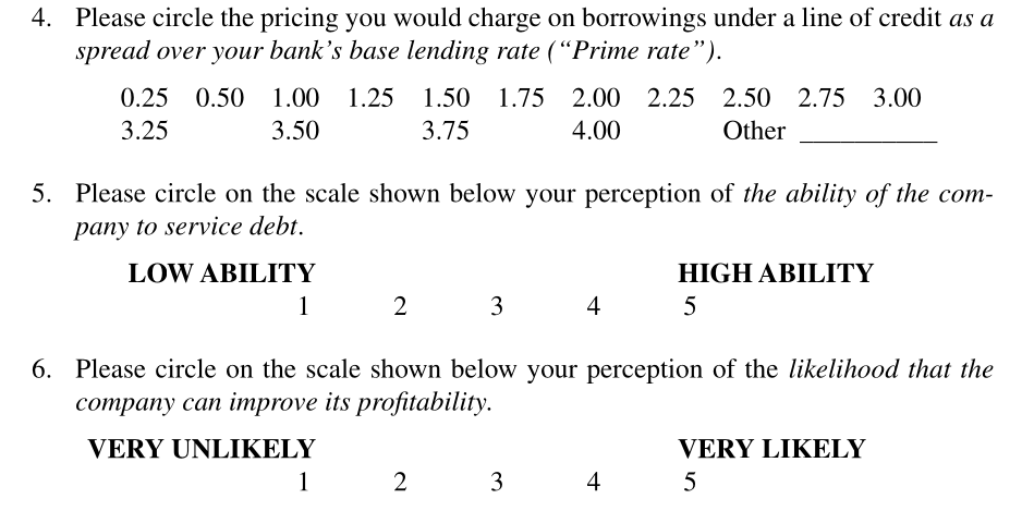

Why use MANOVA?

1. Control experimentwise error
   • do a single test instead of $J$ univariate ANOVAs, thereby reducing the type I error
2. Detect differences in combination that would not be found with univariate tests
3. Increase power (context dependent)

Multivariate model

Postulate the following model: $$Y_{ij}\sim {Normal}_p({\mu }_j,\Sigma ),j=1,\dots J$$

Each response $Y_{ij}$ is $p$-dimensional.

The model is fitted using multivariate linear regression.

Model fitting with multivariate response

In R, we fit a model binding the different vectors of response in a matrix with $p$ columns

data(AVC02, package = "hecedsm")
# Fit the model binding variables with cbind
# on left of tilde (~) symbol
modMANOVA <- manova(
  cbind(prime, debt, profitability) ~ format, 
  data = AVC02)Copy Code

Bivariate MANOVA

Confidence intervals and confidence regions

Model assumptions

The more complex the model, the more assumptions...

Same as ANOVA, with in addition

• The response follow a multivariate normal distribution
  • Shapiro–Wilk test, univariate Q-Q plots
• The covariance matrix is the same for all subjects
  • Box's $M$ test is often used, but highly sensitive to departures from the null (other assumptions impact the test)

When to use MANOVA?

In addition, for this model to make sense, you need just enough correlation (Goldilock principle)

• if correlation is weak, use univariate analyses
  • (no gain from multivariate approach relative to one-way ANOVAs)
  • less power due to additional covariance parameter estimation
• if correlation is too strong, redundancy
  • don't use Likert scales that measure a similar dimension (rather, consider PLS or factor analysis)

Only combine elements that theoretically or conceptually make sense together.

Testing equality of mean vectors

The null hypothesis is that the $J$ groups have the same mean

• $H_0:{\mu }_1=\cdots ={\mu }_J$ against the alternative that at least one vector is different from the rest.

• The null imposes $(J-1)\times p$ restrictions on the parameters.

The test statistic is Hotelling's $T^2$ (with associated null distribution), but we can compute using an $F$ distribution.

Choice of test statistic

In higher dimensions, with $J\ge 3$, there are many statistics that can be used to test equality of mean.

The statistics are constructed from within/between sum covariance matrices.

These are

• Roy's largest root (most powerful provided all assumptions hold)
• Wilk's $\Lambda$: most powerful, most commonly used
• Pillai's trace: most robust choice for departures from normality or equality of covariance matrices

Most give similar conclusion, and they are all equivalent with $J=2$.

Results for MANOVA

summary(modMANOVA) # Pilai is defaultCopy Code

##            Df  Pillai approx F num Df den Df Pr(>F)
## format      2 0.02581  0.55782      6    256 0.7637
## Residuals 129Copy Code

summary(modMANOVA, test = "Wilks")Copy Code

##            Df   Wilks approx F num Df den Df Pr(>F)
## format      2 0.97424   0.5561      6    254  0.765
## Residuals 129Copy Code

summary(modMANOVA, test = "Hotelling-Lawley")Copy Code

##            Df Hotelling-Lawley approx F num Df den Df Pr(>F)
## format      2         0.026397  0.55434      6    252 0.7664
## Residuals 129Copy Code

summary(modMANOVA, test = "Roy") # not reliable here?Copy Code

##            Df      Roy approx F num Df den Df Pr(>F)
## format      2 0.024436   1.0426      3    128 0.3761
## Residuals 129Copy Code

MANOVA for repeated measures

We can also use MANOVA for repeated measures to get away from the hypothesis of equal variance per group or equal correlation.

model <- afex::aov_ez(
  id = "id",           # subject id
  dv = "latency",      # response
  within = "stimulus", # within-subject
  data = hecedsm::AA21,
  fun_aggregate = mean)
model$Anova # for models fitted via 'afex'Copy Code

Output

## 
## Type III Repeated Measures MANOVA Tests: Pillai test statistic
##             Df test stat approx F num Df den Df    Pr(>F)    
## (Intercept)  1   0.95592   238.56      1     11 8.373e-09 ***
## stimulus     1   0.09419     0.52      2     10    0.6098    
## ---
## Signif. codes:  0 '***' 0.001 '**' 0.01 '*' 0.05 '.' 0.1 ' ' 1Copy Code

Follow-up analyses

Researchers often conduct post hoc univariate tests using univariate ANOVA. In R, Holm-Bonferonni's method is applied for marginal tests (you need to correct for multiple testing!)

# Results for univariate analysis of variance (as follow-up)
summary.aov(modMANOVA)
# Note the "rep.meas" as default name 
# to get means of each variable separately
emmeans::emmeans(modMANOVA, specs = c("format", "rep.meas"))Copy Code