Introduction to causal inference

# Introduction to causal inference

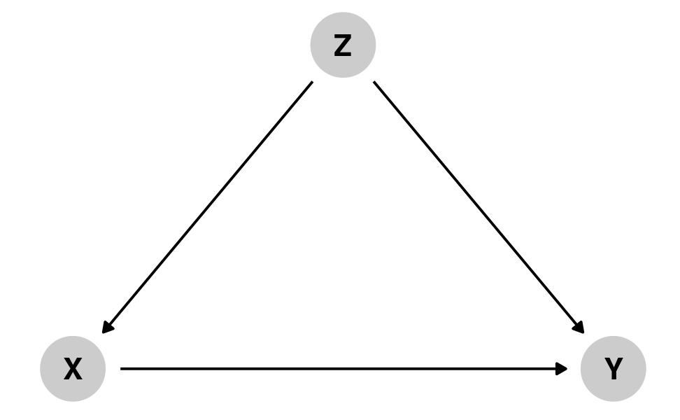
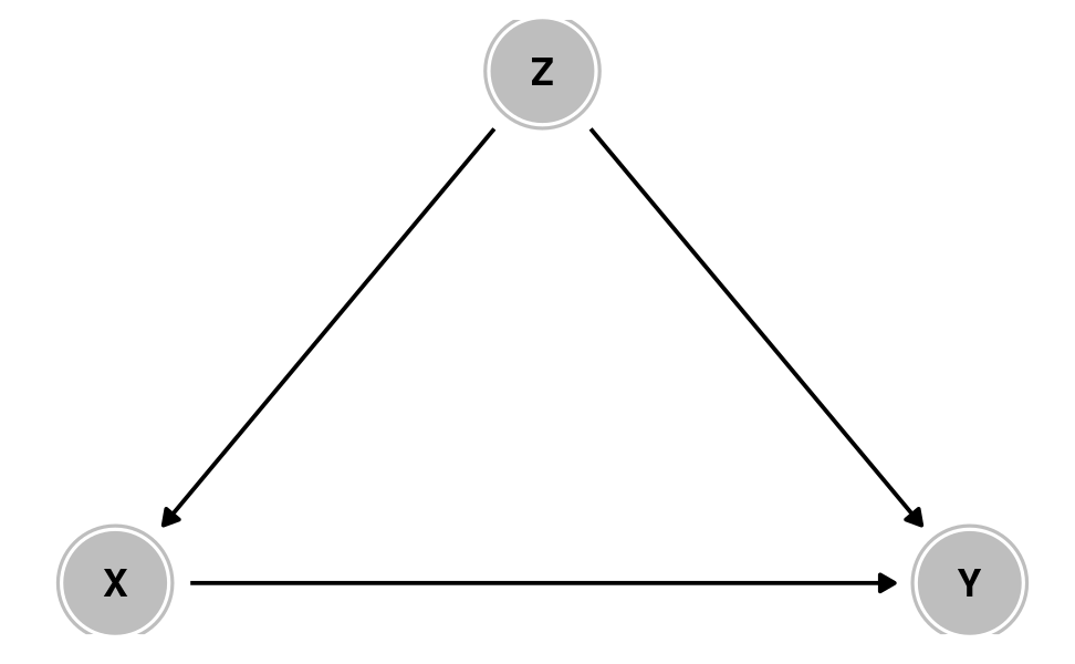
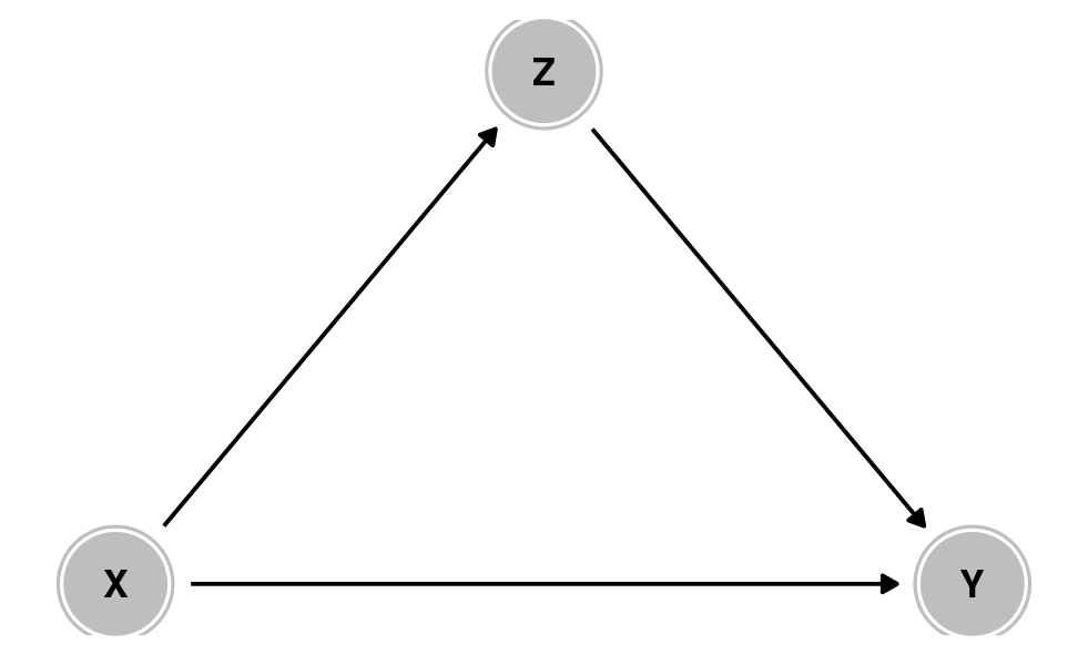
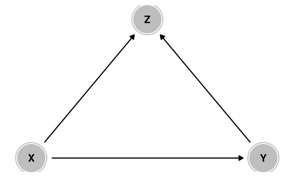
**Session 11**

]

---
name: outline
class: title title-inv-1

# Outline
--

.box-1.large.sp-after-half[Basics of causal inference]
--
.box-2.large.sp-after-half[Directed acyclic graphs]

--
.box-3.large.sp-after-half[Causal mediation]

---

layout: false
name: basicscausal
class: center middle section-title section-title-1

# Causal inference

---

---

# Correlation is not causation

<div class="figure" style="text-align: center">
<img src="img/11/xkcd552_correlation.png" alt="xkcd comic 552 by Randall Munroe, CC BY-NC 2.5 license. Alt text: Correlation doesn't imply causation, but it does waggle its eyebrows suggestively and gesture furtively while mouthing 'look over there'." width="55%" />
<p class="caption">xkcd comic 552 by Randall Munroe, CC BY-NC 2.5 license. Alt text: Correlation doesn't imply causation, but it does waggle its eyebrows suggestively and gesture furtively while mouthing 'look over there'.</p>
</div>
---

# Spurious correlation

<div class="figure" style="text-align: center">
<img src="img/11/5920_per-capita-consumption-of-margarine_correlates-with_the-divorce-rate-in-maine.png" alt="Spurious correlation by Tyler Vigen, licensed under CC BY 4.0" width="60%" />
<p class="caption">Spurious correlation by Tyler Vigen, licensed under CC BY 4.0</p>
</div>

---

# Correlation vs causation

<div class="figure" style="text-align: center">
<img src="img/11/correlation_causation.jpg" alt="Illustration by Andrew Heiss, licensed under CC BY 4.0" width="60%" />
<p class="caption">Illustration by Andrew Heiss, licensed under CC BY 4.0</p>
</div>

---

# Potential outcomes

For individual `\(i\)`, we postulate the existence of a potential outcomes

- `\(Y_i(1)\)` (response for treatment `\(X=1\)`) and 
- `\(Y_i(0)\)` (response for control `\(X=0\)`).

Both are possible, but only one will be realized.

.box-1.medium[Observe outcome for a single treatment]

- Result `\(Y(X)\)` of your test given that you either party `\((X=1)\)` or study `\((X=0)\)` the night before your exam.

---

# Fundamental problem of causal inference

With binary treatment `\(X_i\)`, I observe either `\(Y_i \mid \text{do}(X_i=1)\)` or `\(Y_i \mid \text{do}(X_i=0)\)`.

---

# Causal assumptions?

Since we can't estimate individual treatment, we consider the **average** treatment effect (average over population) `\(\mathsf{E}\{Y(1) - Y(0)\}\)`.

The latter can be estimated as

`\begin{align*}
\textsf{ATE} = \underset{\substack{\text{expected response among}\\\text{treatment group}}}{\mathsf{E}(Y \mid X=1)} - \underset{\substack{\text{expected response among}\\\text{control group}}}{\mathsf{E}(Y \mid X=0)}
\end{align*}`

When is this a valid causal effect?

---

# (Untestable) assumptions

For the ATE to be equivalent to `\(\mathsf{E}\{Y(1) - Y(0)\}\)`, the following are sufficient:

1. *ignorability*, which states that potential outcomes are independent  of assignment to treatment
2. lack of interference: the outcome of any participant is unaffected by the treatment assignment of other participants.
3. consistency: given a treatment `\(X\)` taking level `\(j\)`, the observed value for the response `\(Y \mid X=j\)` is equal to the corresponding potential outcome `\(Y(j)\)`.

---

# Directed acyclic graphs

## .color-light-1[Slides by Dr. Andrew Heiss, CC BY-NC 4.0 License.]

---

---

# Types of data

.box-inv-2.medium.sp-after-half[Experimental]

.box-2.sp-after-half[You have control over which units get treatment]

]

.box-inv-2.medium.sp-after-half[Observational]

.box-2.sp-after-half[You don't have control over which units get treatment]

]

---

# Causal diagrams

.box-inv-2.medium.sp-after-half[Directed acyclic graphs (DAGs)]

.box-2.SMALL[**Directed**: Each node has an arrow that points to another node]

.box-2.SMALL[**Acyclic**: You can't cycle back to a node (and arrows only have one direction)]

.box-2.SMALL[**Graph**: A set of nodes (variables) and vertices (arrows indicating interdependence)]

]

]

---

# Causal diagrams

.box-inv-2.medium.sp-after-half[Directed acyclic graphs (DAGs)]

.box-2.SMALL[Graphical model of the process that generates the data]

.box-2.SMALL[Maps your logical model]

]

![](11-slides_files/figure-html/simple-dag-1.png)
]

---

# Three types of associations

.pull-left-3[
.box-2.medium[Confounding]
<img src="11-slides_files/figure-html/confounding-dag-1.png" width="100%" style="display: block; margin: auto;" />

.box-inv-2.small[Common cause]
]

.pull-middle-3.center[
.box-2.medium[Causation]

.box-inv-2.small[Mediation]
]

.box-inv-2.small[Selection /<br>endogeneity]
]

---

# Confounding

.pull-left-wide[
<img src="11-slides_files/figure-html/confounding-dag-big-1.png" width="100%" style="display: block; margin: auto;" />
]

.box-inv-2.medium.sp-after-half[But **Z** causes both **X** and **Y**]

.box-inv-2.medium.sp-after-half[**Z** * confounds* the **X** → **Y** association]
]

---

# Confounder: effect of money on elections
.box-inv-2.medium.sp-after-half[What are the paths<br>between **money** and **win margin**?]
.pull-left[
<img src="11-slides_files/figure-html/money-elections-1.png" width="100%" style="display: block; margin: auto;" />
]

.box-2.sp-after-half[Money ← Quality → Margin]

.box-inv-2.sp-after-half[Quality is a *confounder*]
]

---

# Experimental data

Since we randomize assignment to treatment `\(X\)`, all arrows **incoming** in `\(X\)` are removed.

With observational data, we need to explicitly model the relationship and strip out the effect of `\(X\)` on `\(Y\)`.

---

# How to adjust with observational data

- Include covariate in regression
- Matching: pair observations that are more alike in each group, and compute difference between these 
- Stratification: estimate effects separately for subpopulation (e.g., young and old, if age is a confounder)
- Inverse probability weighting: estimate probability of self-selection in treatment group, and reweight outcome.

---

# Causation

.pull-left-wide[
<img src="11-slides_files/figure-html/causation-dag-big-1.png" width="100%" style="display: block; margin: auto;" />
]

.box-inv-2.medium.sp-after-half[**X** causes<br>**Z** which causes **Y**]

.box-2.medium.sp-after-half[**Z** is a mediator]
]

---

# Colliders
.pull-left-wide[
<img src="11-slides_files/figure-html/collider-dag-big-1.png" width="100%" style="display: block; margin: auto;" />
]

.box-inv-2.medium.sp-after-half[**Y** causes **Z**]

.box-2.medium.sp-after-half[Should you control for **Z**?]
]

---

layout: false
.pull-left[
.box-2.medium[Colliders can create<br>fake causal effects]
]
.pull-right[
.box-2.medium[Colliders can hide<br>real causal effects]
]
<img src="11-slides_files/figure-html/bulls-scores-1.png" width="50%" style="display: block; margin: auto;" />

---

---

# Colliders and selection bias

---
# Conditioning on colliders

- [Omnipresent in the literature](https://doi.org/10.1146/annurev-soc-071913-043455)

- [Example: When and how does the number of children affect marital satisfaction? An international survey](https://doi.org/10.1371/journal.pone.0249516)
- [Example: The Predictive Validity of the GRE Across Graduate Outcomes](https://doi.org/10.1080/00221546.2023.2187177)

???

A new collider bias teaching example. Sample selects on marriage (not divorced) so: satisfaction ––> [not divorced] <–– children (Richard McElreath, Apr 26, 2021 on Twitter)

Example of confounder: 
https://doi.org/10.1177/109467051454314

---

# Three types of associations

![](11-slides_files/figure-html/confounding-dag-1.png)
.box-inv-2.small.sp-after-half[Common cause]
.box-inv-2.small[Causal forks **X** ← **Z** → **Y**]
]
.pull-middle-3[
.box-2.medium[Causation]
![](11-slides_files/figure-html/mediation-dag-1.png)
.box-inv-2.small.sp-after-half[Mediation]
.box-inv-2.small[Causal chain **X** → **Z** → **Y**]
]
.pull-right-3[
.box-2.medium[Collision]
![](11-slides_files/figure-html/collision-dag-1.png)
.box-inv-2.small.sp-after-half[Selection /<br>endogeneity]
.box-inv-2.small[inverted fork **X** →  **Z** ← **Y**]
]

---

# Life is inherently complex

Source: Andrew Heiss (?), likely from

McQuire, C., Daniel, R., Hurt, L. et al. The causal web of foetal alcohol spectrum disorders: a review and causal diagram. Eur Child Adolesc Psychiatry 29, 575–594 (2020). https://doi.org/10.1007/s00787-018-1264-3