---
title: "MATH 80667A - Week 3"
author: "Léo Belzile"
format: html
eval: true
echo: true
message: false
warning: false
code-tools:
source: true
toggle: false
caption: "Download Quarto file"
---
```{r}
#| echo: false
options(scipen = 100, digits = 3)
```
```{r}
library(dplyr)
library(ggplot2)

data(arithmetic, package = "hecedsm")
## #Fit one way analysis of variance
model <- aov(data = arithmetic,
            formula = score ~ group)
anova(model) #print anova table
# Compute p-value by hand
pf(15.27,
   df1 = 4,
   df2 = 40,
   lower.tail = FALSE)
```
```{r}
#| label: bootstrap-sim
#| cache: true
# How reliable is this F benchmark? To see this, we generate data from a normal
# distribution with the same mean and variance as the original data
mu <- mean(arithmetic$score)
sigma <- sd(arithmetic$score)
B <- 10000L # Number of replications
set.seed(1234) # fix the dice to get reproducible results
pval <- test <- numeric(B) # container to store results
for(b in 1:B){
  # Generate fake results (assuming common average) from normal distribution
  fakescore <- rnorm(n = 45, mean = mu, sd = sigma)
  # For each fake dataset, compute ANOVA F-test statistic and p-value
  out <- anova(aov(fakescore ~ arithmetic$group))
  test[b] <- broom::tidy(out)$statistic[1]
  pval[b] <- broom::tidy(out)$p.value[1]
}
```
```{r}
#| label: fig-histogram-benchmark
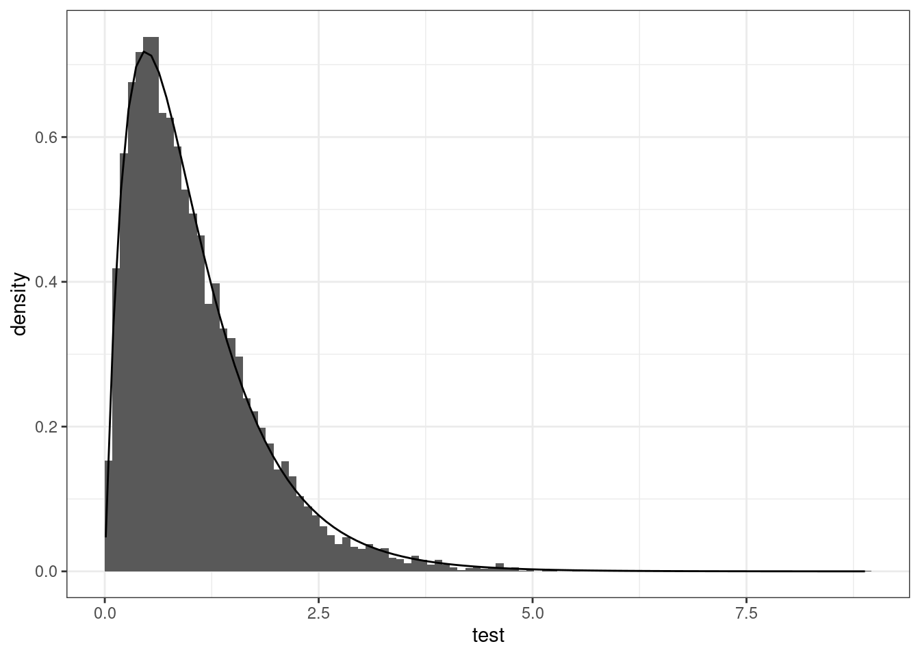
#| fig-cap: "Histogram of bootstrap null distribution against $F(4, 40)$ large-sample approximation."
# Look at what happens under the null
# Histogram (suitably rescaled) matches F(4, 40) benchmark null distribution
ggplot(data = data.frame(test),
       mapping = aes(x = test)) +
  geom_histogram(mapping = aes(y = after_stat(density)),
                 bins = 100L,
                 boundary = 0) +
  stat_function(fun = df, args = list(df1 = 4, df2 = 40)) +
  theme_bw()
```
```{r}
#| label: fig-histogram-pvalues
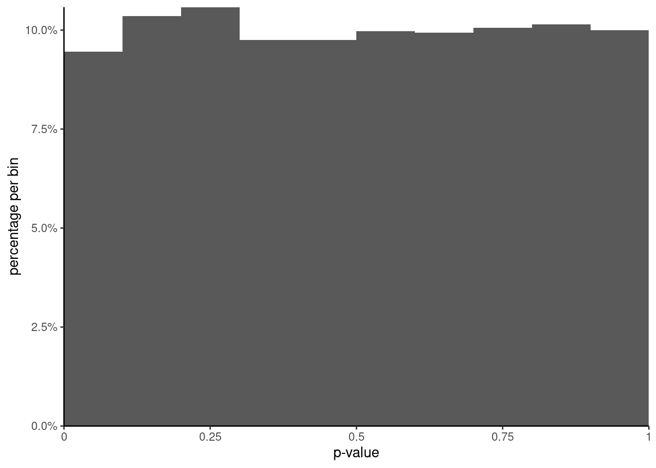
#| fig-cap: "Histogram of $p$-values from the $F$ test."
# When there are no difference in mean and the variance are equal
# i.e., when all assumptions are met, then p-values should be uniformly
# distributed, meaning any number between [0,1] is equally likely
ggplot(data = data.frame(pval),
       mapping = aes(x = pval,
                     y = after_stat(count / sum(count)))) +
  geom_histogram(breaks = seq(0, 1, by = 0.1)) +
  scale_y_continuous(labels = scales::percent,
                     limits = c(0, NA),
                     expand = expansion()) +
  scale_x_continuous(breaks = seq(0, 1, by = 0.25),
                     labels = c("0","0.25","0.5","0.75","1"),
                     limits = c(0, 1), expand = expansion()) +
  labs(y = "percentage per bin", x = "p-value") +
  theme_classic()
```
```{r}
# Two-sample t-test (equal variance) and one-way ANOVA
# are equivalent for comparison of two groups
data("BJF14_S1", package = "hecedsm")
anova(model)
t.test(pain ~ condition, data = BJF14_S1, var.equal = TRUE)
## Tests for equality of variance are simply analysis of variance
## models with different data
car::leveneTest(model, center = median)
# Brown-Forsythe by default, which centers by median
# replace 'center=median' by 'center=mean' to get Levene's test

meds <- arithmetic |>
  group_by(group) |>
  summarize(med = median(score)) # replace by mean to get the result for leveneTest
# Compute absolute difference between response and group median
arithmetic$std <- abs(arithmetic$score - rep(meds$med, each = 9))
# Compute F-test statistic for analysis of variance with the 'new data'
anova(aov(std ~ group, data = arithmetic))
```
```{r}
#| label: tbl-groupmeans
#| tbl-cap: "Average score on arithmetic test per experimental group."
# Parametrization of the linear models (see course notes)
# Here, each group has the same subsample size (balanced)
# So calculations are more intuitive...
data(arithmetic, package = "hecedsm")
# If you fit a one-way ANOVA in R with a linear model via 'lm'
# The default parametrization is such that the intercept corresponds
# to the mean of the first level (alphanumerical order) of the factor
# and other coefficients are difference to that group
arithmetic |>
  dplyr::group_by(group) |>
  dplyr::summarize(meanscore = mean(score)) |>
  knitr::kable(digits = 3,
               col.names = c("group", "mean score"))
```
```{r}
anova1 <- lm(score ~ group, data = arithmetic)
coef(anova1)
# Here, control 1 is baseline (omitted).
# the difference between intercept and control1 is zero, so no coef. reported

# If we change the 'contrast' argument, we can get the "DEFAULT" parametrization
# of analysis of variance models: sum-to-zero.
# In that case, the intercept is the global mean and the sum of
# differences to the mean is zero
anova2 <- lm(score ~ group,
   contrasts = list(group = "contr.sum"),
   data = arithmetic)
# Global mean
as.numeric(coef(anova2)["(Intercept)"])
mean(arithmetic$score)
# Get mean for omitted group (ignore)
# since the sum of differences to the mean is zero
# If we add this coefficient to the global mean, we retrieve the
# subgroup average of 'ignore'
coef(anova2)["(Intercept)"] - sum(coef(anova2)[-1])
```