One-way analysis of variance

Videos

The R code created in the video can be downloaded here and the SPSS code here.

There’s a set of videos that walks through each section below. To make it easier for you to jump around the video examples, I cut the long video into smaller pieces and included them all in one YouTube playlist.

You can also watch the playlist (and skip around to different sections) here:

Notebook

This notebook shows the various manipulation that an experimenter may undertake to test whether the population averages are the same based on some experimental data.

Recall the setup of Example 1.

Hypothesis testing

We can begin by testing whether the group average for the initial measurements at the beginning of the study, prior to any treatment) have the same mean. Strong indication against this null hypothesis would be evidence of a potential problem with the randomization. We compute the one-way analysis of variance table, which includes quantities that enter the F-statistic (named after its large-sample null distribution, which is an F-distribution).¹

We use the lm function function to fit the model: an analysis of variance is a special case of linear model, in which the explanatory variables are categorical variables. The first argument of the function is a formula response ~ treatment, where treatment is the factor or categorical variable indicating the treatment.

The function anova is a method: when applied to the result of a call to lm, it produces an analysis of variance table including among other things the following information:

the value of the test statistic (F value)
the between and within sum of square (these are quantities that enter in the formula of the statistic)
the degrees of freedom of the F null distribution (column Df): these specify the parameters of the large-sample approximation for the null distribution, which is our default benchmark.
the mean square, which are sum of squares divided by the degrees of freedom.
The p-value (Pr(>F)), which gives the probability of observing an outcome as extreme if there was no difference.

We need to decide beforehand the level of the test (typically 5% or lower): this is the percentage of times we will reject the null hypothesis when its true based on observing an extreme outcome. We are asked to perform a binary decision (reject or fail to reject): if the p-value is less than the level, we ‘reject’ the null hypothesis of equal (population) means.

Code

data(BSJ92, package = 'hecedsm')
mod_pre <- aov(formula = pretest1 ~ group,
                     data = BSJ92)
anova_tab <- broom::tidy(anova(mod_pre))
# Save the output in a tibble to get more meaningful column names
# Elements include `statistic`, `df`, `p.value`

Analysis of variance table for pre-test 1
Terms	Degrees of freedom	Sum of squares	Mean square	Statistic	p-value
group	2	20.58	10.288	1.13	0.33
Residuals	63	572.45	9.087

There isn’t strong evidence of difference in strength between groups prior to intervention. We can report the findings as follows:

We carried a one-way analysis for the pre-test results to ensure that the group abilities are the same in each treatment group; results show no significant differences at the 5% level ($F$ (2, 63) = 1.13, $p$ = 0.329).

A similar result for the scores of the first post-test as response variable lead to strong evidence of difference between teaching methods.

Analysis of variance table for post-test 1
Terms	Degrees of freedom	Sum of squares	Mean square	Statistic	p-value
group	2	108.12	54.061	5.32	0.01
Residuals	63	640.50	10.167

Contrasts and estimated marginal means

While the $F$ test may strongly indicate that the means of each group are different, it doesn’t indicate which group is different from the rest. Because we can compare different groups doesn’t mean these comparisons are of any scientific interest and going fishing by looking at all pairwise differences is not necessarily the best strategy.

Code

library(emmeans) #load package
mod_post <- aov(posttest1 ~ group, data = BSJ92)
emmeans_post <- emmeans(object = mod_post, 
                        specs = "group")

Estimated group averages with standard errors and 95% confidence intervals for post-test 1.
Terms	Marginal mean	Standard error	Degrees of freedom	Lower limit (CI)	Upper limit (CI)
DR	6.68	0.68	63	5.32	8.04
DRTA	9.77	0.68	63	8.41	11.13
TA	7.77	0.68	63	6.41	9.13

Thus, we can see that DRTA has the highest average, followed by TA and directed reading (DR). The purpose of Baumann et al. (1992) was to make a particular comparison between treatment groups. From the abstract:

The primary quantitative analyses involved two planned orthogonal contrasts—effect of instruction (TA + DRTA vs. 2 x DRA) and intensity of instruction (TA vs. DRTA)—for three whole-sample dependent measures: (a) an error detection test, (b) a comprehension monitoring questionnaire, and (c) a modified cloze test.

A contrast is a particular linear combination of the different groups, i.e., a sum of weighted mean the coefficients of which sum to zero. To test the hypothesis of Baumann et al. (1992) and writing $\mu$ to denote the population average, we have $\mathscr{H}_0: \mu_{\mathrm{TA}} + \mu_{\mathrm{DRTA}} = 2 \mu_{\mathrm{DRA}}$ or rewritten slightly \[\begin{align*} \mathscr{H}_0: - 2 \mu_{\mathrm{DR}} + \mu_{\mathrm{DRTA}} + \mu_{\mathrm{TA}} = 0. \end{align*}\] with weights $(-2, 1, 1)$; the order of the levels for the treatment are ($\mathrm{DRA}$, $\mathrm{DRTA}$, $\mathrm{TA}$) and it must match that of the coefficients. An equivalent formulation is $(2, -1, -1)$ or $(1, -1/2, -1/2)$: in either case, the estimated differences will be different (up to a constant multiple or a sign change). The vector of weights for $\mathscr{H}_0: \mu_{\mathrm{TA}} = \mu_{\mathrm{DRTA}}$ is, e.g.,($0$, $-1$, $1$): the zero appears because the first component, $\mathrm{DRA}$ doesn’t appear. The two contrasts are orthogonal: these contrasts are special because the tests use disjoint bits of information about the sample.²

Code

# Identify the order of the level of the variables
with(BSJ92, levels(group))

[1] "DR"   "DRTA" "TA"

Code

# DR, DRTA, TA (alphabetical)
contrasts_list <- list(
  "C1: DRTA+TA vs 2DR" = c(-2, 1, 1), 
  # Contrasts: linear combination of means, coefficients sum to zero
  # 2xDR = DRTA + TA => -2*DR + 1*DRTA + 1*TA = 0 and -2+1+1 = 0
  "C1: average (DRTA+TA) vs DR" = c(-1, 0.5, 0.5), 
  #same thing, but halved so in terms of average
  "C2: DRTA vs TA" = c(0, 1, -1),
  "C2: TA vs DRTA" = c(0, -1, 1) 
  # same, but sign flipped
)
contrasts_post <- 
  contrast(object = emmeans_post,
           method = contrasts_list)
contrasts_summary_post <- summary(contrasts_post)

Estimated contrasts for post-test 1.
Contrast	Estimate	Standard error	Degrees of freedom	t statistic	p-value
C1: DRTA+TA vs 2DR	4.18	1.67	63	2.51	0.01
C1: average (DRTA+TA) vs DR	2.09	0.83	63	2.51	0.01
C2: DRTA vs TA	2.00	0.96	63	2.08	0.04
C2: TA vs DRTA	-2.00	0.96	63	-2.08	0.04

We can look at these differences; since DRTA versus TA is a pairwise difference, we could have obtained the $t$-statistic directly from the pairwise contrasts using pairs(emmeans_post). Note that the two different ways of writing the comparison between DR and the average of the other two methods yield different point estimates, but same inference (same $p$-values). For contrast $C_{1b}$, we get half the estimate (but the standard error is also halved) and likewise for the second contrasts we get an estimate of $\mu_{\mathrm{DRTA}} - \mu_{\mathrm{TA}}$ in the first case ($C_2$) and $\mu_{\mathrm{TA}} - \mu_{\mathrm{DRTA}}$: the difference in group averages is the same up to sign.

What is the conclusion of our analysis of contrasts? It looks like the methods involving teaching aloud have a strong impact on reading comprehension relative to only directed reading. The evidence is not as strong when we compare the method that combines directed reading-thinking activity and thinking aloud.

Multiple testing

In this example, we computed two contrasts (excluding the equivalent formulations) so since these comparisons are planned, we could provide the $p$-values as is. However, if we had computed many more tests, it would make sense to account for these so as not to inflate type I error (judicial mistake consisting in sending an innocent to jail).

Code

contrasts_list <- list(
  "C1: DRTA+TA vs 2DR" = c(-2, 1, 1), 
  "C2: DRTA vs TA" = c(0, 1, -1)
)
contrasts_post_scheffe <- 
  contrast(object = emmeans_post,
           method = contrasts_list,
           adjust = "scheffe") # for arbitrary contrasts
# extract p-values
pvals_scheffe <- summary(contrasts_post_scheffe)$p.value
pvals_scheffe

[1] 0.04951625 0.12333575

Code

# Compute Bonferroni and Holm-Bonferroni correction
contrasts_post <- 
  contrast(object = emmeans_post,
           method = contrasts_list,
           adjust = "none") #default for custom contrasts
raw_pval <- summary(contrasts_post)$p.value
p.adjust(p = raw_pval, method = "bonferroni")

[1] 0.02920552 0.08313211

Code

p.adjust(p = raw_pval, method = "holm") #Bonferroni-Holm method

[1] 0.02920552 0.04156606

If we look at the p-values with the Scheffé’s method for custom contrasts, we get 0.015 for contrast 1 and 0.042 for contrast 2: since we are only making two tests here, these are much bigger than the $p$-values from Holm’s method which are 0.03 and 0.04. To try and avoid making type I error, we need to be more stringent to decide on rejection and this translates into bigger $p$-values, so lower power to detect. Try to use the less stringent method that still controls for the family wise error rate to preserve your power!

Model assumptions

Since we have no repeated measurements and there were no detectable difference apriori between students, we can postulate that the records are independent.

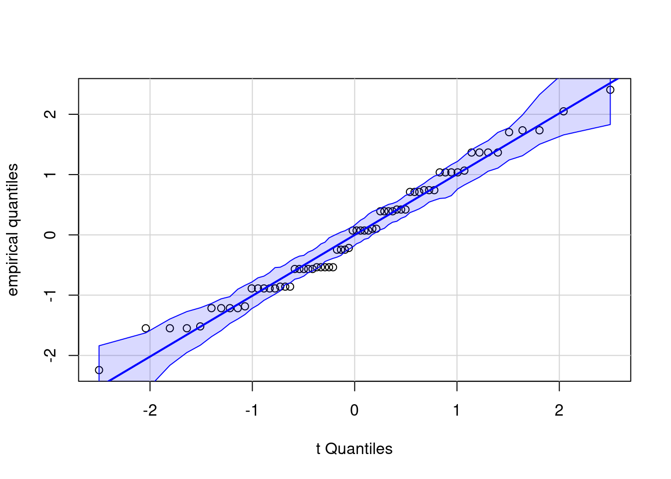
We could test whether the variance are equal: in this case, there is limited evidence of unequal variance. The data are of course not normal (because they consist of the counts of the number of insertions detected by pupils, which are integer-valued). However, we can see if there are extreme values and whether the residuals are far from normal. The simulated quantile-quantile plot shows that all points more or less align with the straight line and all fall within the confidence intervals, so there is no problem with this normality assumption (which anyway matters little).

Are measurements additive? After assigning the pre-test 1, the experimenters adjusted the scale and made the post-test harder to avoid having maximum scores (considering that students also were more experienced).

Because the students performed at a higher-than-expected level on Pretest 1 (61% of all intruded sentences were correctly identified), the experimenters were concerned about a potential post-intervention ceiling effect on this posttest, an occurrence which could mask group differences. To reduce the likelihood of a ceiling effect, the intruded sentences for Posttest 1 were written so their inconsistencies were more subtle than those included in Pretest 1, which explains the somewhat lower level of performance on Posttest 1 (51% of all intruded sentences correctly identified).

This seems to have been successful since the maximum score is 15 out of 16 intrusions, while there were two students who scored 16 on the pre-test.

The next step is checking that the variability is the same in each group. Assuming equal variance is convenient because we can use more information (the whole sample) to estimate the level of uncertainty rather than solely the observations from each group. The more observations we use to estimate the variance, the more reliable our measure is (assuming that the variance were equal in each group to begin with).

Code

# test for equality of variance
car::leveneTest(posttest1 ~ group, data = BSJ92)

Levene's Test for Homogeneity of Variance (center = median)
      Df F value Pr(>F)
group  2  2.1297 0.1273
      63

Code

# Quantile-quantile plot
car::qqPlot(x = mod_post, # lm object
            ylab = 'empirical quantiles', # change y-axis label
            id = FALSE) # Don't print to console 'outlying' observations

Code

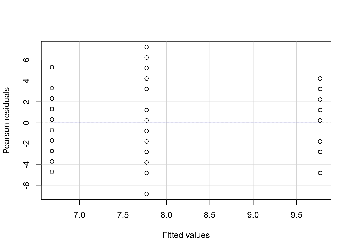
# Residual plot (linearity, but useless for one way ANOVA)
car::residualPlot(mod_post)

If we were worried about the possibility of unequal variances, we could fit the model by estimating the variance separately in each group. This does not materially change the conclusions about teaching methods relative to the directed reading benchmark.

Code

oneway.test(posttest1 ~ group, data = BSJ92)


    One-way analysis of means (not assuming equal variances)

data:  posttest1 and group
F = 6.9878, num df = 2.00, denom df = 41.13, p-value = 0.00244

Auxiliary and concomitant observation

The purpose of a good experimental design is to reduce the variability to better detect treatment effects. In the above example, we could have added a concomitant variable (the pre-test score) that captures the individual variability. This amounts to doing a paired comparison between post- and pre-test results. It helps with the analysis because it absorbs the baseline strength of individual students: by subtracting their records, we get their individual average out of the equation and thus there is less variability.

Code

anova_post_c <- lm(posttest1 ~ offset(pretest1) + group,
                   data = BSJ92) 
anova_tab_c <- broom::tidy(anova(anova_post_c)) #anova table

Compare this ANOVA table with the preceding. We could repeat the same procedure to compute the contrasts.

Using auxiliary information allows one to reduce the intrinsic variability: the estimated variance $\widehat{\sigma}^2$ is 6.66 with the auxiliary information and 9.09 without: since we reduce the level of background noise, we get a higher signal-to-noise ratio. As a result, the p-value for the global test is smaller than with only posttest1 as response.

Analysis of variance table
Terms	Degrees of freedom	Sum of squares	Mean square	Statistic	p-value
group	2	168.21	84.106	12.64	0
Residuals	63	419.32	6.656

References

Baumann, J. F., Seifert-Kessell, N., & Jones, L. A. (1992). Effect of think-aloud instruction on elementary students’ comprehension monitoring abilities. Journal of Reading Behavior, 24(2), 143–172. https://doi.org/10.1080/10862969209547770

Footnotes

The F stands for Fisher, who pioneered much of the work on experimental design.↩︎
This technical term means that the two vectors defining the contrasts are orthogonal: their inner product is thus zero: $(-2 \times 0) + (1 \times -1) + (1 \times 1) = 0$. In practice, we specify contrasts because they answer questions of scientific interest, not because of their fancy mathematical properties.↩︎

--- title: "One-way analysis of variance" type: docs editor_options: chunk_output_type: console --- ```{r slides-videos, echo=FALSE, include=FALSE} source(here::here("R", "youtube-playlist.R")) playlist_id <- "PLUB8VZzxA8IvHyjTG5P7ZfyTQWEUbFhcc" slide_details <- tibble::tribble( ~title, ~youtube_id, "ANOVA table", "7ysgXYx6Rwg", "Contrasts and estimated marginal means", "KJ99KgeApNs", "Multiple testing", "dM1IkaVFy6w", #"Effect size", "hD7HBU1EyDk", #"Power", "W7mUTKruk_s" ) ``` # Videos The **R** code created in the video [can be downloaded here](/example/onewayanova-video.R) and the [SPSS code here](/example/oneway.sps). ```{r show-youtube-list, echo=FALSE, results="asis"} youtube_list(slide_details, playlist_id, example = TRUE) ``` # Notebook This notebook shows the various manipulation that an experimenter may undertake to test whether the population averages are the same based on some experimental data. Recall the setup of [Example 1](/example/introduction.html). ```{r setup, include = FALSE} library(knitr) options(knitr.kable.NA = '') options(tidyverse.quiet = TRUE) library(tidyverse) data(BSJ92, package = 'hecedsm') suppressPackageStartupMessages(library(effectsize)) ``` ## Hypothesis testing We can begin by testing whether the group average for the initial measurements at the beginning of the study, prior to any treatment) have the same mean. Strong indication against this null hypothesis would be evidence of a potential problem with the randomization. We compute the one-way analysis of variance table, which includes quantities that enter the _F_-statistic (named after its large-sample null distribution, which is an _F_-distribution).^[The _F_ stands for Fisher, who pioneered much of the work on experimental design.] We use the `lm` function function to fit the model: an analysis of variance is a special case of linear model, in which the explanatory variables are categorical variables. The first argument of the function is a formula `response ~ treatment`, where `treatment` is the factor or categorical variable indicating the treatment. The function `anova` is a method: when applied to the result of a call to `lm`, it produces an analysis of variance table including among other things the following information: 1) the value of the test statistic (`F value`) 2) the between and within sum of square (these are quantities that enter in the formula of the statistic) 3) the degrees of freedom of the _F_ null distribution (column `Df`): these specify the parameters of the large-sample approximation for the null distribution, which is our default benchmark. 4) the mean square, which are sum of squares divided by the degrees of freedom. 5) The _p_-value (`Pr(>F)`), which gives the probability of observing an outcome as extreme if there was no difference. We need to decide beforehand the level of the test (typically 5\% or lower): this is the percentage of times we will reject the null hypothesis when its true based on observing an extreme outcome. We are asked to perform a binary decision (reject or fail to reject): if the _p_-value is less than the level, we 'reject' the null hypothesis of equal (population) means. ```{r anova-stat, echo = TRUE, eval = TRUE} data(BSJ92, package = 'hecedsm') mod_pre <- aov(formula = pretest1 ~ group, data = BSJ92) anova_tab <- broom::tidy(anova(mod_pre)) # Save the output in a tibble to get more meaningful column names # Elements include `statistic`, `df`, `p.value` ``` ```{r print-anova-table, echo = FALSE, results = 'asis'} knitr::kable(anova_tab, digits = c(2,2,2,3), caption = "Analysis of variance table for pre-test 1", col.names = c("Terms", "Degrees of freedom", "Sum of squares", "Mean square", "Statistic", "p-value")) |> kableExtra::kable_styling(position = "center") ``` There isn't strong evidence of difference in strength between groups prior to intervention. We can report the findings as follows: We carried a one-way analysis for the pre-test results to ensure that the group abilities are the same in each treatment group; results show no significant differences at the 5\% level ($F$ (`r anova_tab$df[1]`, `r anova_tab$df[2]`) = `r round(anova_tab$statistic[1], 2)`, $p$ = `r format.pval(anova_tab$p.value[1], digits = 3, eps=1e-3)`). A similar result for the scores of the first post-test as response variable lead to strong evidence of difference between teaching methods. ```{r linmod2, echo = FALSE, eval = TRUE} mod_post <- aov(posttest1 ~ group, data = BSJ92) anova_post <- broom::tidy(anova(mod_post)) ``` ```{r print-anova-table-post, echo = FALSE, results = 'asis'} knitr::kable(anova_post, digits = c(2,2,2,3), caption = "Analysis of variance table for post-test 1", col.names = c("Terms", "Degrees of freedom", "Sum of squares", "Mean square", "Statistic", "p-value"),) |> kableExtra::kable_styling(position = "center") ``` ## Contrasts and estimated marginal means While the $F$ test may strongly indicate that the means of each group are different, it doesn't indicate which group is different from the rest. Because we can compare different groups doesn't mean these comparisons are of any scientific interest and going fishing by looking at all pairwise differences is not necessarily the best strategy. ```{r pairwise-baumann, echo = TRUE, eval = TRUE} library(emmeans) #load package mod_post <- aov(posttest1 ~ group, data = BSJ92) emmeans_post <- emmeans(object = mod_post, specs = "group") ``` ```{r print-pairwise, echo = FALSE, eval = TRUE} kable(emmeans_post, digits = c(2,2,2,0,2,2), caption = "Estimated group averages with standard errors and 95% confidence intervals for post-test 1.", col.names = c("Terms", "Marginal mean", "Standard error", "Degrees of freedom", "Lower limit (CI)", "Upper limit (CI)")) |> kableExtra::kable_styling(position = "center") ``` Thus, we can see that `DRTA` has the highest average, followed by `TA` and directed reading (`DR`). The purpose of @Baumann:1992 was to make a particular comparison between treatment groups. From the abstract: > The primary quantitative analyses involved two planned orthogonal contrasts—effect of instruction (TA + DRTA vs. 2 x DRA) and intensity of instruction (TA vs. DRTA)—for three whole-sample dependent measures: (a) an error detection test, (b) a comprehension monitoring questionnaire, and (c) a modified cloze test. A **contrast** is a particular linear combination of the different groups, i.e., a sum of weighted mean the coefficients of which sum to zero. To test the hypothesis of @Baumann:1992 and writing $\mu$ to denote the population average, we have $\mathscr{H}_0: \mu_{\mathrm{TA}} + \mu_{\mathrm{DRTA}} = 2 \mu_{\mathrm{DRA}}$ or rewritten slightly $$\begin{align*} \mathscr{H}_0: - 2 \mu_{\mathrm{DR}} + \mu_{\mathrm{DRTA}} + \mu_{\mathrm{TA}} = 0. \end{align*}$$ with weights $(-2, 1, 1)$; the order of the levels for the treatment are ($\mathrm{DRA}$, $\mathrm{DRTA}$, $\mathrm{TA}$) and it must match that of the coefficients. An equivalent formulation is $(2, -1, -1)$ or $(1, -1/2, -1/2)$: in either case, the estimated differences will be different (up to a constant multiple or a sign change). The vector of weights for $\mathscr{H}_0: \mu_{\mathrm{TA}} = \mu_{\mathrm{DRTA}}$ is, e.g.,($0$, $-1$, $1$): the zero appears because the first component, $\mathrm{DRA}$ doesn't appear. The two contrasts are orthogonal: these contrasts are special because the tests use disjoint bits of information about the sample.^[This technical term means that the two vectors defining the contrasts are orthogonal: their inner product is thus zero: $(-2 \times 0) + (1 \times -1) + (1 \times 1) = 0$. In practice, we specify contrasts because they answer questions of scientific interest, not because of their fancy mathematical properties.] ```{r contrasts, echo = TRUE, eval = TRUE} # Identify the order of the level of the variables with(BSJ92, levels(group)) # DR, DRTA, TA (alphabetical) contrasts_list <- list( "C1: DRTA+TA vs 2DR" = c(-2, 1, 1), # Contrasts: linear combination of means, coefficients sum to zero # 2xDR = DRTA + TA => -2*DR + 1*DRTA + 1*TA = 0 and -2+1+1 = 0 "C1: average (DRTA+TA) vs DR" = c(-1, 0.5, 0.5), #same thing, but halved so in terms of average "C2: DRTA vs TA" = c(0, 1, -1), "C2: TA vs DRTA" = c(0, -1, 1) # same, but sign flipped ) contrasts_post <- contrast(object = emmeans_post, method = contrasts_list) contrasts_summary_post <- summary(contrasts_post) ``` ```{r print-contrasts, echo = FALSE, eval = TRUE} kable(contrasts_post, digits = c(2,2,2,0,2,2), caption = "Estimated contrasts for post-test 1.", col.names = c("Contrast", "Estimate", "Standard error", "Degrees of freedom", "t statistic", "p-value")) |> kableExtra::kable_styling(position = "center") ``` We can look at these differences; since `DRTA` versus `TA` is a pairwise difference, we could have obtained the $t$-statistic directly from the pairwise contrasts using `pairs(emmeans_post)`. Note that the two different ways of writing the comparison between `DR` and the average of the other two methods yield different point estimates, but same inference (same $p$-values). For contrast $C_{1b}$, we get half the estimate (but the standard error is also halved) and likewise for the second contrasts we get an estimate of $\mu_{\mathrm{DRTA}} - \mu_{\mathrm{TA}}$ in the first case ($C_2$) and $\mu_{\mathrm{TA}} - \mu_{\mathrm{DRTA}}$: the difference in group averages is the same up to sign. What is the conclusion of our analysis of contrasts? It looks like the methods involving teaching aloud have a strong impact on reading comprehension relative to only directed reading. The evidence is not as strong when we compare the method that combines directed reading-thinking activity and thinking aloud. ## Multiple testing In this example, we computed two contrasts (excluding the equivalent formulations) so since these comparisons are planned, we could provide the $p$-values as is. However, if we had computed many more tests, it would make sense to account for these so as not to inflate type I error (judicial mistake consisting in sending an innocent to jail). ```{r contrastsfixed, eval = TRUE, echo = TRUE} contrasts_list <- list( "C1: DRTA+TA vs 2DR" = c(-2, 1, 1), "C2: DRTA vs TA" = c(0, 1, -1) ) contrasts_post_scheffe <- contrast(object = emmeans_post, method = contrasts_list, adjust = "scheffe") # for arbitrary contrasts # extract p-values pvals_scheffe <- summary(contrasts_post_scheffe)$p.value pvals_scheffe # Compute Bonferroni and Holm-Bonferroni correction contrasts_post <- contrast(object = emmeans_post, method = contrasts_list, adjust = "none") #default for custom contrasts raw_pval <- summary(contrasts_post)$p.value p.adjust(p = raw_pval, method = "bonferroni") p.adjust(p = raw_pval, method = "holm") #Bonferroni-Holm method ``` If we look at the _p_-values with the Scheffé's method for custom contrasts, we get `r round(summary(contrasts_post)$p.value[1], 3)` for contrast 1 and `r round(summary(contrasts_post)$p.value[2], 3)` for contrast 2: since we are only making two tests here, these are much bigger than the $p$-values from Holm's method which are `r round(p.adjust(p = raw_pval, method = "holm")[1],2)` and `r round(p.adjust(p = raw_pval, method = "holm")[2],2)`. To try and avoid making type I error, we need to be more stringent to decide on rejection and this translates into bigger $p$-values, so lower power to detect. Try to use the less stringent method that still controls for the family wise error rate to preserve your power! ## Model assumptions Since we have no repeated measurements and there were no detectable difference apriori between students, we can postulate that the records are independent. We could test whether the variance are equal: in this case, there is limited evidence of unequal variance. The data are of course not normal (because they consist of the counts of the number of insertions detected by pupils, which are integer-valued). However, we can see if there are extreme values and whether the residuals are far from normal. The simulated quantile-quantile plot shows that all points more or less align with the straight line and all fall within the confidence intervals, so there is no problem with this normality assumption (which anyway matters little). Are measurements additive? After assigning the pre-test 1, the experimenters adjusted the scale and made the post-test harder to avoid having maximum scores (considering that students also were more experienced). > Because the students performed at a higher-than-expected level on Pretest 1 (61% of all intruded sentences were correctly identified), the experimenters were concerned about a potential post-intervention ceiling effect on this posttest, an occurrence which could mask group differences. To reduce the likelihood of a ceiling effect, the intruded sentences for Posttest 1 were written so their inconsistencies were more subtle than those included in Pretest 1, which explains the somewhat lower level of performance on Posttest 1 (51% of all intruded sentences correctly identified). This seems to have been successful since the maximum score is `r max(BSJ92$posttest1)` out of 16 intrusions, while there were two students who scored 16 on the pre-test. The next step is checking that the variability is the same in each group. Assuming equal variance is convenient because we can use more information (the whole sample) to estimate the level of uncertainty rather than solely the observations from each group. The more observations we use to estimate the variance, the more reliable our measure is (assuming that the variance were equal in each group to begin with). ```{r testequalvariance, echo = TRUE, eval = TRUE} # test for equality of variance car::leveneTest(posttest1 ~ group, data = BSJ92) # Quantile-quantile plot car::qqPlot(x = mod_post, # lm object ylab = 'empirical quantiles', # change y-axis label id = FALSE) # Don't print to console 'outlying' observations # Residual plot (linearity, but useless for one way ANOVA) car::residualPlot(mod_post) ``` If we were worried about the possibility of unequal variances, we could fit the model by estimating the variance separately in each group. This does not materially change the conclusions about teaching methods relative to the directed reading benchmark. ```{r welch, echo = TRUE, eval = TRUE} oneway.test(posttest1 ~ group, data = BSJ92) ``` ## Auxiliary and concomitant observation The purpose of a good experimental design is to reduce the variability to better detect treatment effects. In the above example, we could have added a concomitant variable (the pre-test score) that captures the individual variability. This amounts to doing a paired comparison between post- and pre-test results. It helps with the analysis because it absorbs the baseline strength of individual students: by subtracting their records, we get their individual average out of the equation and thus there is less variability. ```{r concomitant, eval = TRUE, echo = TRUE} anova_post_c <- lm(posttest1 ~ offset(pretest1) + group, data = BSJ92) anova_tab_c <- broom::tidy(anova(anova_post_c)) #anova table ``` Compare this ANOVA table with the preceding. We could repeat the same procedure to compute the contrasts. Using auxiliary information allows one to reduce the intrinsic variability: the estimated variance $\widehat{\sigma}^2$ is `r round(anova_tab_c$meansq[2],2)` with the auxiliary information and `r round(anova_tab$meansq[2],2)` without: since we reduce the level of background noise, we get a higher signal-to-noise ratio. As a result, the _p_-value for the global test is smaller than with only `posttest1` as response. ```{r printanovaConcomitant, echo = FALSE, eval = TRUE} knitr::kable(anova_tab_c, digits = c(2,2,2,3), caption = "Analysis of variance table", col.names = c("Terms", "Degrees of freedom", "Sum of squares", "Mean square", "Statistic", "p-value")) |> kableExtra::kable_styling(position = "center") ``` ## References