The following demonstration explains how to compute repeated measures ANOVA that include within-subject factors. Download the R code or the SPSS code. Such models can also be fitted using linear mixed models, see the R code or the SPSS code for a demonstration.
There’s a set of videos that walks through each section below. To make it easier for you to jump around the video examples, I cut the long video into smaller pieces and included them all in one YouTube playlist.
We consider Experiment 3 from Hatano et al. (2022). The data consist in a two by two mixed analysis of variance. The authors studied engagement and enjoyment from waiting tasks, and “potential effects of time interval on the underestimation of task motivation by manipulating the time for the waiting task”. The waiting time was randomly assigned to either short (3 minutes) or long (20 minutes) with equal probability, but participants were either told that there was a 70% chance of being assigned to the short session, or 30% chance.
Data
We first load the data from the package and inspect the content.
# Number of people in each groupwith(HOSM22_E3, table(waiting)/2)
waiting
 long short
   32    31
From this, we can see that there each student is assigned to a single waiting time, but that they have both rating types. Since there are 63 students, the study is unbalanced but by a single person; this may be due to exclusions.
Model fitting
We use the afex package (analysis of factorial design) with the aov_ez. We need to specify the identifier of the subjects (id), the response variable (dv) and both between- (between) and within-subject (within) factors. Each of those names must be quoted (strings)
Code
options(contrasts =c("contr.sum", "contr.poly"))fmod <- afex::aov_ez(id ="id", dv ="imscore", between ="waiting",within ="ratingtype",data = HOSM22_E3)anova(fmod)
Type III Repeated Measures MANOVA Tests: Pillai test statistic
                   Df test stat approx F num Df den Df    Pr(>F)
(Intercept)         1   0.89286   508.37      1     61 < 2.2e-16 ***
waiting             1   0.15577    11.26      1     61   0.00137 **
ratingtype          1   0.38652    38.43      1     61 5.388e-08 ***
waiting:ratingtype  1   0.00134     0.08      1     61   0.77575
---
Signif. codes:  0 '***' 0.001 '**' 0.01 '*' 0.05 '.' 0.1 ' ' 1
The output includes the \(F\)-tests for the two main effects and the interaction and global effect sizes \(\widehat{\eta}^2\) (ges). There is no output for tests of sphericity, since there are only two measurements per person and thus a single mean different within-subject (so the test to check equality doesn’t make sense with a single number). We could however compare variance between groups using Levene’s test
Notice that the degrees of freedom for the denominator of the test are based on the number of participants, here 63.
Example 2
Study 5 of Halevy & Berson (2022) aimed to demonstrate that events in the distant future rather than the near future influenced the prospect of peace, along with the degree of abstractness. The experimental design is a
2 (current state: war vs. peace) by 2 (predicted outcome: war vs. peace) by 2 (temporal distance: next year vs. twenty years into the future) mixed design
with current state and predicted outcome as between-subject factors and temporal distance as within-subject factor. The response is the estimated likelihood of each outcome on a 7-point Likert scale ranging from extremely unlikely (1) to extremely likely (7). Data are presented in long-format. The question asked was of the form
There is currently [war/peace] between the two tribes in Velvetia. Thinking about [next year/in 20 years], how likely is it that there will be [war/peace] in Velvetia?
We begin by loading the data and looking at the repartition of the measurements over conditions for the between-subject factors:
Code
data(HB22_S5, package ="hecedsm")xtabs(~ curstate + predout, data = HB22_S5)
        predout
curstate peace war
   peace   148 164
   war     118 124
The data is unbalanced, but there are sufficient measurements in each condition.
Again, there is no output for the test of sphericity and no difference with the multivariate analysis of variance model because each measurement per person has it’s own variance and correlation parameter, but there is a single comparison for the likelihood scores (for the temporal distance).
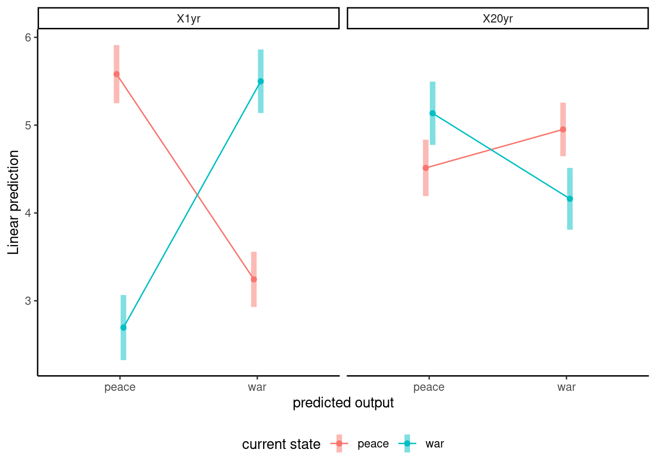
Since the three-way interaction is statistically significant, we need to compare each cell within the levels of the other factor: for example, we could fix the temporal horizon to 1 year and compare the predictions based on both current state and predicted outcome.
Code
library(emmeans)
Welcome to emmeans.
Caution: You lose important information if you filter this package's results.
See '? untidy'
The interaction plot suggest quite strongly that the difference in the reaction is much more pronounced score-wise for short-term horizon predictions than for the long-run. The authors commented this finding by stating
when the current state is characterized by war (intergroup conflict), peace is seen as significantly more likely in the distant future than in the near future. In contrast, when the current state is characterized by peace, war is seen as significantly more likely in the distant future than in the near future.
References
Halevy, N., & Berson, Y. (2022). Thinking about the distant future promotes the prospects of peace: A construal-level perspective on intergroup conflict resolution. Journal of Conflict Resolution, 66(6), 1119–1143. https://doi.org/10.1177/00220027221079402
Hatano, A., Ogulmus, C., Shigemasu, H., & Murayama, K. (2022). Thinking about thinking: People underestimate how enjoyable and engaging just waiting is. Journal of Experimental Psychology: General, 151(12), 3213–3229. https://doi.org/10.1037/xge0001255
Source Code
---title: "Repeated measure ANOVA"type: docseditor_options: chunk_output_type: console---The following demonstration explains how to compute repeated measures ANOVA that include within-subject factors. Download the [**R** code](/example/repeated.R) or the [SPSS code](/example/repeated.sps). Such models can also be fitted using linear mixed models, see the [**R** code](/example/repeatedwmixedmodels.R) or the [SPSS code](/example/repeatedwmixedmodels.sps) for a demonstration.```{r slides-videos, echo=FALSE, include=FALSE}source(here::here("R", "youtube-playlist.R"))playlist_id <-"PLUB8VZzxA8IucBRbpQTZCF5GzJX2KUVfp"slide_details <- tibble::tribble(~title, ~youtube_id,"One-way within design", "tJ0O4uUJMis","Two-way mixed design", "mJ7-_mjoaHo","Three-way mixed design", "VKGDHscj0P0")```# VideosThe **R** code created in the video [can be downloaded here](/example/repeated.R) and the [SPSS code here](/example/repeated.sps).```{r show-youtube-list, echo=FALSE, results="asis"}youtube_list(slide_details, playlist_id, example =TRUE)```You can also watch SPSS videos:- [Repeated measures](https://www.youtube.com/watch?v=VPck9Z8m9hc&list=PLUB8VZzxA8Iv41lUAoTRNoat3oCVlFY62)- [Repeated measures (within-between design)](https://www.youtube.com/watch?v=1eVVFziSN_k&list=PLUB8VZzxA8Iv41lUAoTRNoat3oCVlFY62)# Example 1We consider Experiment 3 from @Hatano:2022. The data consist in a two by two mixed analysis of variance. The authors studied engagement and enjoyment from waiting tasks, and "potential effects of time interval on the underestimation of task motivation by manipulating the time for the waiting task". The waiting time was randomly assigned to either short (3 minutes) or long (20 minutes) with equal probability, but participants were either told that there was a 70% chance of being assigned to the short session, or 30% chance.## Data We first load the data from the package and inspect the content.```{r}data(HOSM22_E3, package ="hecedsm")str(HOSM22_E3)# Number of people in each groupwith(HOSM22_E3, table(waiting)/2)```From this, we can see that there each student is assigned to a single waiting time, but that they have both rating types. Since there are 63 students, the study is unbalanced but by a single person; this may be due to exclusions.## Model fittingWe use the `afex` package (analysis of factorial design) with the `aov_ez`. We need to specify the identifier of the subjects (`id`), the response variable (`dv`) and both between- (`between`) and within-subject (`within`) factors. Each of those names must be quoted (strings)```{r}options(contrasts =c("contr.sum", "contr.poly"))fmod <- afex::aov_ez(id ="id", dv ="imscore", between ="waiting",within ="ratingtype",data = HOSM22_E3)anova(fmod)# MANOVA testsfmod$Anova```The output includes the $F$-tests for the two main effects and the interaction and global effect sizes $\widehat{\eta}^2$ (`ges`). There is no output for tests of sphericity, since there are only two measurements per person and thus a single mean different within-subject (so the test to check equality doesn't make sense with a single number). We could however compare variance between groups using Levene's testNotice that the degrees of freedom for the denominator of the test are based on the number of participants, here `r length(unique(HOSM22_E3$id))`.# Example 2Study 5 of @Halevy.Berson:2022 aimed to demonstrate that events in the distant future rather than the near future influenced the prospect of peace, along with the degree of abstractness. The experimental design is a > 2 (current state: war vs. peace) by 2 (predicted outcome: war vs. peace) by 2 (temporal distance: next year vs. twenty years into the future) mixed designwith current state and predicted outcome as between-subject factors and temporal distance as within-subject factor. The response is the estimated likelihood of each outcome on a 7-point Likert scale ranging from extremely unlikely (1) to extremely likely (7). Data are presented in long-format. The question asked was of the form >There is currently [war/peace] between the two tribes in Velvetia. Thinking about [next year/in 20 years], how likely is it that there will be [war/peace] in Velvetia?We begin by loading the data and looking at the repartition of the measurements over conditions for the between-subject factors:```{r}data(HB22_S5, package ="hecedsm")xtabs(~ curstate + predout, data = HB22_S5)```The data is unbalanced, but there are sufficient measurements in each condition.```{r}mmod <- afex::aov_ez(id ="id",dv ="likelihood",between =c("curstate","predout"),within ="tempdist",data = HB22_S5)summary(mmod)```Again, there is no output for the test of sphericity and no difference with the multivariate analysis of variance model because each measurement per person has it's own variance and correlation parameter, but there is a single comparison for the likelihood scores (for the temporal distance).Since the three-way interaction is statistically significant, we need to compare each cell within the levels of the other factor: for example, we could fix the temporal horizon to 1 year and compare the predictions based on both current state and predicted outcome.```{r}library(emmeans)library(ggplot2)emm <-emmeans(mmod, specs =c("curstate","predout"),by ="tempdist")emmip(emm, formula = curstate ~ predout | tempdist,CIs =TRUE) +theme_classic() +theme(legend.position ="bottom") +labs(x ="predicted output",color ="current state")```The interaction plot suggest quite strongly that the difference in the reaction is much more pronounced score-wise for short-term horizon predictions than for the long-run. The authors commented this finding by stating> when the current state is characterized by war (intergroup conflict), peace is seen as significantly more likely in the distant future than in the near future. In contrast, when the current state is characterized by peace, war is seen as significantly more likely in the distant future than in the near future.